import os
import logging
import matplotlib.pyplot as plt
import numpy as np
import pandas as pd
from IPython import display

%matplotlib widget
if not os.getenv(
    "NBGRADER_EXECUTION"
):
    %reload_ext jupyter_ai
In this notebook, you will use Weka to compare different classifiers trained using different algorithms and parameters.
Noise Curve
Complete the tutorial exercises in [Witten11] Ex 17.2.6 to 17.2.11 using the dataset glass.arff described at the beginning of [Witten11] 17.2.
The video below demonstrates how to use the Explorer interface to train 3-Nearest-Neighbor (3NN) classifier with 50% of the training data corrupted by noise.
Weka provides a convenient interface, called the Experimenter, to compare the performances of different classification algorithms on different datasets. This is demonstrated by the video below.
A more flexible way is to use the python-weka-wrapper3. First, run the following to start the java virtual machine and load the glass.arff dataset:
import weka.core.jvm as jvm
from weka.classifiers import Classifier, Evaluation, FilteredClassifier
from weka.core.classes import Random
from weka.core.converters import Loader
from weka.filters import Filter

jvm.start(logging_level=logging.ERROR)
loader = Loader(classname="weka.core.converters.ArffLoader")
data = loader.load_url(
    "https://raw.githubusercontent.com/Waikato/weka-3.8/master/wekadocs/data/"
    + "glass.arff"
)
data.class_is_last()
We can then create a filtered classifier with the following tools:
from weka.classifiers import Classifier, Evaluation, FilteredClassifier
from weka.core.classes import Random
from weka.filters import Filter
add_noise = Filter(classname="weka.filters.unsupervised.attribute.AddNoise")
IBk = Classifier(classname="weka.classifiers.lazy.IBk")
fc = FilteredClassifier()
fc.filter = add_noise
fc.classifier = IBkTo compute the 10-fold cross-validated accuracy of 3-NN classification with 50% noise:
add_noise.options = ["-P", str(50), "-S", str(0)]  # percentage noise  # random seed
IBk.options = ["-K", str(3)]  # number of nearest neighbors
evl = Evaluation(data)
evl.crossvalidate_model(fc, data, 10, Random(1))
evl.percent_correctnoise_df = pd.DataFrame(columns=["k=1", "k=3", "k=5"], dtype=float)
noise_df.insert(0, "Percentage Noise", np.arange(0, 101, 10))
# YOUR CODE HERE
raise NotImplementedError
display.display(noise_df.round(2))
plt.figure(num=1, figsize=(8, 5), clear=True)
for k in ["1", "3", "5"]:
plt.plot(
noise_df["Percentage Noise"], noise_df["k=" + k], label="k=" + k, marker="o"
)
plt.legend()
plt.xlabel("Percentage Noise")
plt.ylabel("Accuracies")
plt.title(r"Training IB$k$ on noisy data for different $k$")
plt.show()%%ai
Explain in a paragraph how the noise curve can show whether a learning algorithm
is prone to overfitting.YOUR ANSWER HERE
YOUR ANSWER HERE
%%ai
Explain in a paragraph whether it is possible to overfit even when the training
data has no noise, which is defined as the irregularity irrelevant to the
general pattern?
Training Curve
train_df = pd.DataFrame(columns=["IBk", "J48"], dtype=float)
train_df.insert(0, "Percentage of Training Set", np.arange(10, 101, 10))

# YOUR CODE HERE
raise NotImplementedError

display.display(train_df.round(2))

plt.figure(num=3, figsize=(8, 5), clear=True)
for clf in ["IBk", "J48"]:
    plt.plot(
        train_df["Percentage of Training Set"], train_df[clf], label=clf, marker="o"
    )
plt.legend()
plt.xlabel("Percentage of Training Set")
plt.ylabel("Accuracies")
plt.title(r"Training IB$k$ and J48 with different amount of data")
plt.show()%%ai
Explain in a paragraph how the training curve can show whether a learning
algorithm is prone to underfitting.YOUR ANSWER HERE
YOUR ANSWER HERE
YOUR ANSWER HERE
%%ai
Explain in a paragraph whether it is always possible to find the best fit
for a given training data.
Classification Boundaries
Complete the tutorial exercises in [Witten11] Ex 17.3.1 to 17.3.6 using the boundary visualizer for different classifiers on iris.2D.arff (NOT iris.arff) dataset.
For OneR, note that the boundary is decided based on two conditions in Appendix A of Holte93:
(3a) Minimum size of the optimal class should be at least
minBucketSize, and(3b) the optimal class of the smallest attribute value just above the boundary should be different from the optimal class just below the boundary.
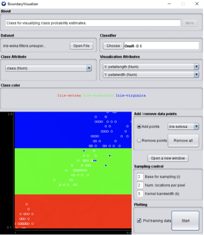
Figure 1:OneR decision boundary
%%ai
Explain the following two rules in deciding how values are partitioned into
intervals so that every interval satisfies the following constraints:
(a) there is at least one class that is "optimal" for more than SMALL of the
    values in the interval. This constraint does not apply to the rightmost
    interval.
(b) If $V[I]$ is the smallest value for attribute $A$ in the training set that
    is larger than the values in interval $I$ then there is no class $C$ that
is optimal both for $V[I]$ and for interval $I$.YOUR ANSWER HERE
YOUR ANSWER HERE
YOUR ANSWER HERE
YOUR ANSWER HERE
YOUR ANSWER HERE
YOUR ANSWER HERE
%%ai
How does Weka's BoundaryVisualizer plot the decision boundaries, especially
when there are more than two input features?