Evaluation with scikit-learn

import os
from functools import lru_cache

import matplotlib.pyplot as plt
import numpy as np
import pandas as pd
from IPython import display
from ipywidgets import IntSlider, interact
from sklearn import datasets, tree
from sklearn.model_selection import (
    StratifiedKFold,
    cross_val_predict,
    cross_val_score,
    train_test_split,
)

%matplotlib widget
if not os.getenv(
    "NBGRADER_EXECUTION"
):
    %load_ext jupyter_ai
    %ai update chatgpt dive:chat
    # %ai update chatgpt dive-azure:gpt4o

In this notebook, you will learn to use the popular Python package scikit-learn to evaluate a classifier. Compared to Weka GUI, the programming language gives a greater flexibility in controlling the learning process.

Data Preparation¶

About the dataset¶

We will use a popular dataset called the iris dataset. Iris is a flower with three different species shown below.

Iris virginica — Figure 3:Iris verginica

The three iris species differ in the lengths and widths of their petals and sepals.

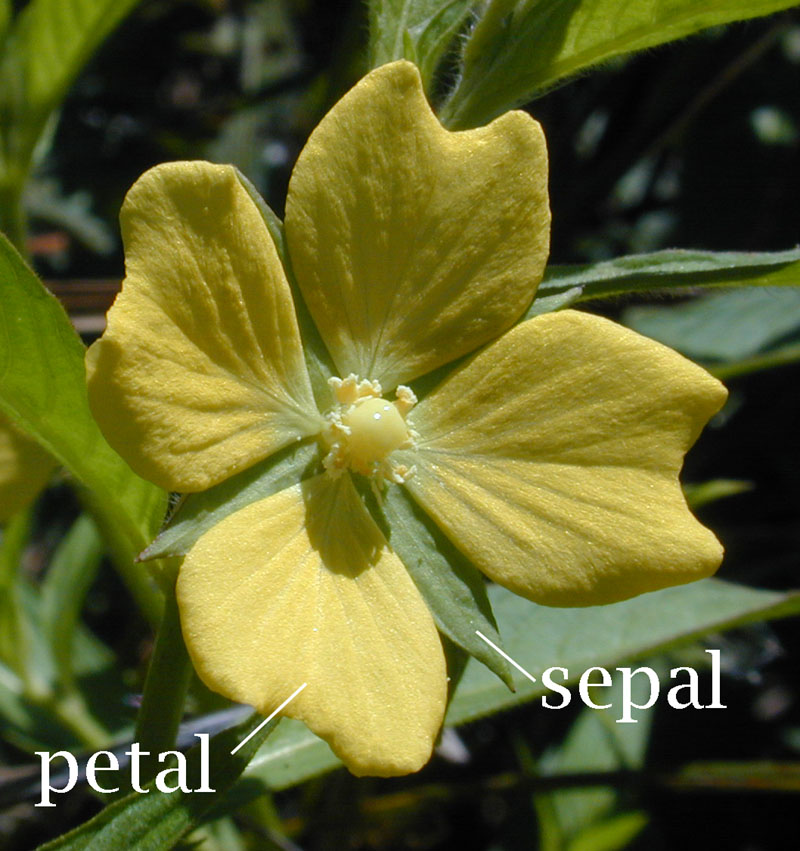
petal and sepal — Figure 4:Petal and sepal of a flower

A standard data mining task is to train a model that can classify the spieces (target) automatically based on the lengths and widths of the petals and sepals (input features).

Load dataset from scikit-learn¶

How to load the iris dataset?

To load the iris dataset, we can simply import the sklearn.datasets package.

from sklearn import datasets

iris = datasets.load_iris()
type(iris)  # object type

sklearn stores the dataset as a Bunch object, which is essentially a bunch of properties put together.

How to learn more about a library?

Detailed documentation can be found at https://scikit-learn.org. You can also learn about the library in the notebook:

# Display the docstring
datasets.load_iris?

Tip

In a notebook, we can get the docstring (document string) of a function conveniently using the symbol ? such as:

datasets.load_iris?

or ?datasets.load_iris, which is the same as running help(datasets.load_iris). You can also display the source code using double question mark ?? such as datasets.load_iris??.

We can also use the contextual help by placing the cursor over a function name and

click the menu item Help->Show Contextual Help or
press the short-cut key Shift + Tab.

How to learn more about the dataset?

The property DESCR (description) is a string that contains some background information about the dataset:

print(iris.DESCR)

All the properties of an object can be listed using the built-in function dir (directory):

dir(iris)

How to show the data?

The properties data and target contains the data values.

type(iris.data), type(iris.target)

The data are stored as numpy array, a powerful data type optimized for performance. It provides useful properties and methods to describe and process the data:

iris.data.shape, iris.data.ndim, iris.data.dtype

To show the input feature names:

iris.feature_names

To show the means and standard deviations of the input features:

iris.data.mean(axis=0), iris.data.std(axis=0)

All the public properties/methods of numpy array are printed below using list comprehension:

import numpy as np  # import numpy and rename it as np

print([attr for attr in dir(np.ndarray) if attr[0] != "_"])
# private attributes starting with underscore are not printed

What is the target feature?

The target variable of the iris dataset is the flower type, whose names are stored by the following property:

iris.target_names

iris.target is an array of integer indices from {0, 1, 2} for the three classes.

iris.target

Exercise 1

Complete the following cell with a tuple of the following properties for the target (instead of input features) of the iris dataset:

shape,
number of dimensions, and
the data types of the values.

# YOUR CODE HERE
raise NotImplementedError
shape, ndim, dtype

Source

# tests
assert (
    isinstance(shape, tuple) and isinstance(ndim, int) and isinstance(dtype, np.dtype)
)

Exercise 2

Fill in the following cell with a tuple of

the list of minimum values of the input features, and
the list of maximum values of the input features.

# YOUR CODE HERE
raise NotImplementedError
feature_min, feature_max

Source

# tests
assert feature_min.shape == (4,) == feature_max.shape

Create pandas DataFrame¶

The package pandas provides additional tools to display and process a dataset. First, we translate the Bunch object into a pandas DataFrame object.

import pandas as pd

# write the input features first
iris_df = pd.DataFrame(data=iris.data, columns=iris.feature_names)

# append the target values to the last column
iris_df["target"] = iris.target

iris_df  # to display the DataFrame

In jupyter notebook, a DataFrame object is conveniently displayed as an HTML table. We can control how much information to show by setting the display options.

We can also display the statistics of different numerical attributes using the method describe and boxplot.

iris_df.describe()

plt.figure(1, clear=True)
iris_df.boxplot()
plt.show()

How to handle nominal class attribute?

Note that the boxplot also covers the target attribute, but it should not. (Why?) Let’s take a look at the current datatypes of the different attributes.

print(iris_df.dtypes)

The target is regarded as a numeric attribute with type integer int64. Instead, the target should be categorical with only three possible values, one for each iris species.

To fix this, we can use the astype method to convert the data type automatically.^[1]

iris_df.target = iris_df.target.astype("category")
iris_df.dtypes

plt.figure(num=2, clear=True)
iris_df.select_dtypes(exclude=['category']).boxplot()
plt.show()

We can also rename the target categories {0, 1, 2} to the more meaningful names of the iris species in iris.target_names.^[2]

iris_df.target = iris_df.target.cat.rename_categories(iris.target_names)
iris_df  # check that the target values are now setosa, versicolor, or virginica.

Exercise 3

For nominal attributes, a more meaningful statistic than the mean is the counts of different possible values. To count the number of instances for each flower class, assign target_counts to the output of the value_counts method of an appropriate column of iris_df.

# YOUR CODE HERE
raise NotImplementedError
target_counts

Source

# tests
assert target_counts.shape == (3,)

How to select rows and columns?

The following uses ipywidgets to demonstrate different ways of selecting (slicing) the rows of a DataFrame:^[3]

from ipywidgets import interact


@interact(
    command=[
        "iris_df.head()",
        "iris_df[0:4]",
        "iris_df.iloc[0:4]",
        "iris_df.loc[0:4]",
        "iris_df.loc[iris_df.index.isin(range(0,4))]",
        "iris_df.loc[lambda df: df.target=='setosa']",
        "iris_df.tail()",
        "iris_df[-1:]",
    ]
)
def select_rows(command):
    output = eval(command)
    display.display(output)

The following demonstrates different ways to slice columns:

@interact(
    command=[
        "iris_df.target",
        'iris_df["target"]',
        'iris_df[["target"]]',
        "iris_df[iris_df.columns[:-1]]",
        "iris_df.loc[:,iris_df.columns[0]:iris_df.columns[-1]]",
        'iris_df.loc[:,~iris_df.columns.isin(["target"])]',
        "iris_df.iloc[:,:-1]",
    ]
)
def select_columns(command):
    output = eval(command)
    display.display(output)

For instance, to compute the mean values of the input features for iris setosa:

iris_df

iris_df.iloc[lambda df: (df["target"] == "setosa").to_numpy(), :-1].mean()

We can also use the method groupby to obtain the mean values by flower types:

iris_df.groupby("target", observed=False).mean()

# YOUR CODE HERE
raise NotImplementedError
iris2d_df

Source

# tests
assert set(iris2d_df.columns) == {"petal length (cm)", "petal width (cm)", "target"}

Alternative methods of loading a dataset¶

The following code loads the iris dataset from an ARFF file instead.

import io
import urllib.request

from scipy.io import arff

ftpstream = urllib.request.urlopen(
    "https://raw.githubusercontent.com/Waikato/weka-3.8/master/wekadocs/data/iris.arff"
)
iris_arff = arff.loadarff(io.StringIO(ftpstream.read().decode("utf-8")))
iris_df2 = pd.DataFrame(iris_arff[0])
iris_df2["class"] = iris_df2["class"].astype("category")
iris_df2

Pandas also provides a method to read the iris dataset directly from a CSV file locally or the internet, such as the UCI respository.

iris_df3 = pd.read_csv(
    "https://archive.ics.uci.edu/ml/machine-learning-databases/iris/iris.data",
    sep=",",
    dtype={"target": "category"},
    header=None,
    names=iris.feature_names + ["target"],
)
iris_df3

The additional arguments dtype, header, and names allow us to specify the attribute datatypes and names.

Training and Testing¶

To obtain unbiased performance estimates of a learning algorithm, the fundamental principle is to use separate datasets for training and testing. If there is only one dataset, we can split it into training sets and test sets by random sampling. In the following subsections, we will illustrate some methods of splitting the datasets for training and testing.

Stratified holdout method¶

The (stratified) holdout method randomly samples data for training or testing without replacement. It is implemented by the train_test_split function from the sklearn.model_selection package.

from sklearn.model_selection import train_test_split

X_train, X_test, Y_train, Y_test = train_test_split(
    iris_df[iris.feature_names],  # We also separated the input features
    iris_df.target,  # and target as X and Y for the training and test sets.
    test_size=0.2,  # fraction for test set
    random_state=1,
    stratify=iris_df.target,
)  # random seed

X_train.shape, X_test.shape, Y_train.shape, Y_test.shape

The fraction of holdout test data is:

len(Y_test) / (len(Y_test) + len(Y_train))

The class proportion of the iris dataset can be plotted as follows:

plt.figure(num=3, clear=True)
iris_df.target.value_counts().plot(kind="bar", ylabel="counts")
plt.show()
_code = In[-1].rsplit(maxsplit=1)[0] # store the code for chatting with LLM

%%ai chatgpt -f text
The label of the x-axis is too long and they got clipped. How to fix?
--
{_code}

We can check the effect of stratification on the class proportions:

@interact(stratify=False, data=["Y_train", "Y_test"], seed=(0, 10))
def plot_class_proportions(stratify, data, seed=0):
    Y_train, Y_test = train_test_split(
        iris_df.target,
        test_size=0.2,
        random_state=seed,
        stratify=iris_df.target if stratify else None,
    )
    plt.figure(num=4, clear=True)
    eval(data).value_counts().sort_index().plot(kind="bar", ylabel="counts")
    plt.xticks(rotation=45, ha='right')
    plt.tight_layout()
    plt.show()

We first apply a learning algorithm, say the decision tree induction algorithm, to train a classifier using only the training set.

from sklearn import tree

clf = tree.DecisionTreeClassifier(random_state=0)  # the training is also randomized
clf.fit(X_train, Y_train)  # fit the model to the training set

We can use the predict method of the trained classifier to predict the flower type from input features.

Y_pred = clf.predict(X_test)
Y_pred

The following code returns the accuracy of the classifier, namely, the fraction of correct predictions on the test set.

accuracy_holdout = (Y_pred == Y_test).mean()
accuracy_holdout

The score method performs essentially the same computation. The following code uses f-string to format the accuracy to 3 decimal places.

print(f"Accuracy: {clf.score(X_test, Y_test):0.3f}")

To see input features of misclassified test instances:

X_test[Y_pred != Y_test]

Source

# YOUR CODE HERE
raise NotImplementedError
accuracy_holdout_training_set

from functools import lru_cache

import numpy as np


@lru_cache(None)  # cache the return value to avoid repeated computation
def holdout_score(seed):
    clf = tree.DecisionTreeClassifier(random_state=seed)
    X_train, X_test, Y_train, Y_test = train_test_split(
        iris_df[iris.feature_names], iris_df.target, test_size=0.2, random_state=seed
    )
    # YOUR CODE HERE
    raise NotImplementedError


@lru_cache(None)
def subsampling_score(N):
    return sum(holdout_score(i) for i in range(N)) / N

Source

# tests
assert np.isclose(subsampling_score(50), 0.9466666666666663)

After implementing subsampling_score, the following code should plot the mean accuracies for different N. Check that the variation becomes smaller as N increases.

plt.figure(num=5, clear=True)
plt.stem([subsampling_score(i) for i in range(1, 50)])
plt.xlabel(r"$N$")
plt.ylabel(r"Mean accuracy")
plt.show()

Stratified cross-validation¶

A popular method of evaluating a classification algorithm is to randomly partition the data into $k$ folds, which are nearly equal-sized blocks of instances. The score is the average of the accuracies obtained by using each fold to test a classifier trained using the remaining folds.

The module sklearn.model_selection provides two functions cross_val_predict and cross_val_score for this purpose.

from sklearn.model_selection import StratifiedKFold, cross_val_predict, cross_val_score

cv = StratifiedKFold(n_splits=5, random_state=0, shuffle=True)

For instance, the following returns the misclassified instances by 5-fold cross-validation.

iris_df["prediction"] = pd.Categorical(
    cross_val_predict(clf, iris_df[iris.feature_names], iris_df.target, cv=cv)
)
iris_df.loc[lambda df: df["target"] != df["prediction"]]

clf = tree.DecisionTreeClassifier(random_state=0)
scores = cross_val_score(clf, iris_df[iris.feature_names], iris_df.target, cv=5)
print("Accuracies: ", ", ".join(f"{acc:.4f}" for acc in scores))
print(f"Mean accuracy: {scores.mean():.4f}")

# YOUR CODE HERE
raise NotImplementedError
accuracy_cv