Evaluation for Skewed Dataset

import logging
import os

import numpy as np
import pandas as pd
import weka.core.jvm as jvm
import weka.plot.classifiers as plcls
from weka.classifiers import Classifier, Evaluation
from weka.core.classes import Random
from weka.core.converters import Loader

%matplotlib widget
if not os.getenv(
    "NBGRADER_EXECUTION"
):
    %load_ext jupyter_ai
    %ai update chatgpt dive:chat
    # %ai update chatgpt dive-azure:gpt4o

Class imbalance problem¶

In this notebook, we will analyze a skewed dataset for detecting microcalcifications in mammograms. The goal is to build a classifier to identify whether a bright spot in a mammogram is a micro-calcification (an early sign of breast cancer).

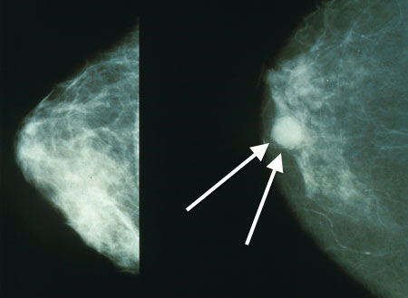
Mammo breast cancer — Figure 1:Micro-calcification

The dataset can be downloaded from OpenML in ARFF format. The following loads the data using python-weka-wrapper3.

jvm.start(logging_level=logging.ERROR)

loader = Loader(classname="weka.core.converters.ArffLoader")
data = loader.load_url("https://www.openml.org/data/download/52214/phpn1jVwe")
data.class_is_last()
print(data.summary(data))

A set of 24 mammograms was segmented to locate small bright spots, which are candidates for classifying malignant clusters of micro-calcifications. There are 7 attributes and over 11,000 instances.^[1]

%%ai chatgpt -f text
Explain each of the following attributes of the mammogram dataset in one line:
- Area (number of pixels)
- Average grey level
- Gradient strength (of perimeter pixels)
- Root mean square noise (fluctuation of the pixel values)
- Root mean square noise of local background
- Contrast (average grey level minus average of a 2-pixel wide border)
- (Low order moment-based) Shape descriptor

To compute the 10-fold cross-validation accuracy for J48:

clf = Classifier(classname="weka.classifiers.trees.J48")
evl = Evaluation(data)
evl.crossvalidate_model(clf, data, 10, Random(1))

print(f"Accuracy: {evl.percent_correct:.3g}%")

You should see that the accuracy is close to 100%. To show the confusion matrix:

confusion_matrix = pd.DataFrame(
    evl.confusion_matrix,
    dtype=int,
    columns=[f'predicted class "{v}"' for v in data.class_attribute.values],
    index=[f'class "{v}"' for v in data.class_attribute.values],
)
confusion_matrix

Each row of the confusion matrix corresponds to a class value (1: malignant, -1: benign), and each column corresponds to a predicted class. Each entry is a count of instances belonging to a specific class and having a particular predicted class.

# YOUR CODE HERE
raise NotImplementedError
print(f"Percentage of malignant detected: {percent_of_malignant_detected:.3g}%")

Different Performance Metrics¶

In a skewed dataset, very high accuracy can be achieved using ZeroR, which predicts the majority class regardless of input feature values. Therefore, it is essential to use additional performance metrics to properly train and evaluate a classification algorithm.

The table below lists the values of TP, TN, FP, and FN:

pos_class = 1  # specify the postive class value
TP = evl.num_true_positives(pos_class)
FN = evl.num_false_negatives(pos_class)
FP = evl.num_false_positives(pos_class)
TN = evl.num_true_negatives(pos_class)

TFPN = pd.DataFrame(
    [[TP, FN], [FP, TN]],
    dtype=int,
    columns=["predicted +ve", "predicted -ve"],
    index=["+ve", "-ve"],
)
TFPN

This is similar to a confusion matrix, where the entries represent the counts of instances with columns as actual values and rows as predicted values. A confusion matrix is more general because it:

does not specify a positive class, and
can have more than two rows/columns in multi-class classification problems.

To return the precision, recall, and specificity:

performance = {
    "precision": evl.precision(pos_class),
    "recall": evl.recall(pos_class),
    "specificity": evl.true_negative_rate(pos_class),
}

assert np.isclose(performance["precision"], TP / (TP + FP))
assert np.isclose(performance["recall"], TP / (TP + FN))
assert np.isclose(performance["specificity"], TN / (TN + FP))

performance

The precision and recall are below 80% and 60% respectively:

If a bright spot is classified as malignant, the chance it is malignant is less than 80%.
Out of all malignant bright spots, less than 60% are identified as malignant.

Despite this, the specificity is nearly perfect, i.e.,

close to 100% benign bright spots are identified as benign.

This high specificity is primarily because most bright spots are benign, not because the classifier effectively distinguishes between malignant and benign spots.

# YOUR CODE HERE
raise NotImplementedError
print(f"negative predictive value (NPV): {performance['NPV']:.3g}")

The following give other measures that capture the performance in both precision and recall:

Definition 2 (

F

-scores)

$F_{\beta}$ -score is defined as

\begin{align} F_{\beta} &:= \left( \frac{\precision^{-1} + \beta^2 \cdot \recall^{-1}}{\beta^2 + 1}\right)^{-1}\\ &= \frac{(\beta^2+1)\cdot \precision\cdot \recall }{\beta^2\precision + \recall}. \end{align}

(2)

$F$ -score is the special case when $\beta=1$ ,

\begin{align} F := F_1 &= \left( \frac{\precision^{-1} + \recall^{-1}}{2}\right)^{-1} \\ &= \frac{2\cdot \precision\cdot \recall }{\precision + \recall}, \end{align}

(3)

which is the harmonic mean of precision and recall.

$F$ -scores are useful in training a classifier to maximize both precision and recall because it is the harmonic mean of precision and recall. The harmonic mean is small if any of its components are small.

performance["F"] = evl.f_measure(pos_class)
print(f"F-score: {performance['F']:.3g}")

%%ai chatgpt -f text
Explain why the F-score is low if either precision or recall is low.

# YOUR CODE HERE
raise NotImplementedError
print(f"F_2 score: {performance['F_2']:.3g}")

%%ai chatgpt -f text
How have problems in information retrieval motivated the use of the 
F-beta score instead of the F-score?

Exercise 4

Using ZeroR as the classifier, assign to ZeroR_performance a dictionary of precision, recall, and specificity. You can create the dictionary as follows:

ZeroR_performance = {
    'precision': ___,
    'recall': ___,
    'specificity': ___
}

Use 10-fold cross-validation with a random seed of 1. If the value is not a number, you may enter it as np.nan.

# YOUR CODE HERE
raise NotImplementedError
ZeroR_performance

YOUR ANSWER HERE

%%ai chatgpt -f text
How does the Kappa statistic help capture performance beyond a 
baseline classifier?

Operating Curves for Probabilistic Classifier¶

For a probabilistic classifier that returns probabilities of different classes, we can obtain a trade-off between precision and recall by changing a threshold γ for positive prediction, i.e., predict positive if and only if the probability estimate for positive class is larger than γ.

To plot the precision-recall curve and prints the area under the curve, we can use the following tool:

import weka.plot.classifiers as plcls

plcls.plot_prc(evl, class_index=[1])
performance["PRC"] = evl.area_under_prc(pos_class)
print(f"area under precision-recall curve (PRC): {performance['PRC']:.3g}")

%%ai chatgpt -f text
Why the PRC curve can have positive slope? Should precision be negatively
related to recall?

YOUR ANSWER HERE

%%ai chatgpt -f text
How is AUC of PRC different from F-score?

We can also plot the ROC (receiver operator characteristics) curve to show the trade-off between recall (true positive rate) and false positive rate:

plcls.plot_roc(evl, class_index=[1])
performance["AUC"] = evl.area_under_roc(pos_class)
print(f"area under ROC curve (AUC): {performance['AUC']:.3g}")

YOUR ANSWER HERE

%%ai chatgpt -f text
How is AUC under ROC different from AUC under PRC?

Footnotes¶

For more details on the dataset, refer to Section 4 of the original paper (Woods et al. 1993).
↩

References¶

Woods, K. S., Solka, J. L., Priebe, C. E., Kegelmeyer, W. P., Doss, C. C., & Bowyer, K. W. (1994). Comparative Evaluation of Pattern Recognition Techniques for Detection of Microcalcifications in Mammography. In State of the Art in Digital Mammographic Image Analysis (pp. 213–231). WORLD SCIENTIFIC. 10.1142/9789812797834_0011

Tutorial 4

Different Classifiers with scikit-learn

Tutorial 5

Training with Skewed Dataset