Density-Based Clustering

import os
import ipywidgets as widgets
import matplotlib.pyplot as plt
import numpy as np
import pandas as pd
import seaborn as sns
from ipywidgets import interact
from sklearn import datasets, preprocessing
from sklearn.cluster import DBSCAN
from sklearn.pipeline import make_pipeline

%matplotlib widget
if not os.getenv(
    "NBGRADER_EXECUTION"
):
    %load_ext jupyter_ai
    %ai update chatgpt dive:chat
    # %ai update chatgpt dive-azure:gpt4o

DBSCAN with scikit-learn¶

DBSCAN (Density-based spatial clustering of applications with noise) is a clustering algorithm that identifies clusters as regions of densely populated instances.

Definition 1 (DBSCAN)

Given the parameters $\varepsilon$ and $\op{MinPts}$ , a point $\M{p}\in D$ in the dataset is called a core point if it satisfies

\begin{align} |D\cap N_{\varepsilon}(\M{p})|&\geq \op{MinPts} \quad \text{where}\\ N_{\varepsilon}(\M{p})&:= \Set{\M{q}\in D| \op{dist}(\M{p},\M{q})\leq \varepsilon}. \end{align}

(1)

The core points form the pillars of the clusters to generate. More precisely, clusters are grown from core points to points in their neighborhood $N_{\varepsilon}(\M{p})$ , referred to as density-reachable points:

A point is regarded as noise if it has no cluster assignment, i.e., not density-reachable from a core point.
A non-core point reachable from a core point is called a border point.

We will create synthetic datasets using the sample generators of sklearn. In particular, we first create spherical clusters using sklearn.datasets.make_blobs:

def XY2df(X, Y):
    """Return a DataFrame for 2D data with 2 input features X and a target Y."""
    df = pd.DataFrame(columns=["feature1", "feature2", "target"])
    df["target"] = Y
    df[["feature1", "feature2"]] = X
    return df

fig, ax = plt.subplots(clear=True, figsize=(10, 10), layout="constrained", num=1)
ax.set_aspect("equal")

@interact
def generate_blobs(
    n_samples=widgets.IntSlider(value=200, min=10, max=1000, continuous_update=False),
    centers=widgets.IntSlider(value=3, min=1, max=4, continuous_update=False),
    cluster_std=widgets.FloatSlider(
        value=0.5, min=0, max=5, step=0.1, continuous_update=False
    ),
):
    df = XY2df(
        *datasets.make_blobs(
            n_samples=n_samples,
            centers=centers,
            cluster_std=cluster_std,
            random_state=0,
        )
    )
    ax.clear()
    sns.scatterplot(data=df, x="feature1", y="feature2", hue="target", ax=ax)
    plt.show()

We will use the dataset df_spherical created with the parameters below:

df_spherical = XY2df(
    *datasets.make_blobs(n_samples=200, centers=3, cluster_std=0.5, random_state=0)
)

To create non-spherical clusters, one way is to use sklearn.datasets.make_circle.

df_nonspherical = XY2df(
    *datasets.make_circles(n_samples=200, factor=0.1, noise=0.1, random_state=0)
)

fig, ax = plt.subplots(clear=True, figsize=(10, 10), layout="constrained", num=2)
ax.set_aspect("equal")

@interact
def generate_circles(
    n_samples=widgets.IntSlider(value=200, min=10, max=1000, continuous_update=False),
    factor=widgets.FloatSlider(
        value=0.1, min=0, max=0.99, step=0.01, continuous_update=False
    ),
    noise=widgets.FloatSlider(
        value=0.1, min=0, max=1, step=0.1, continuous_update=False
    ),
):
    df = pd.DataFrame(columns=["feature1", "feature2", "target"])
    # YOUR CODE HERE
    raise NotImplementedError
    df["target"] = Y
    df[["feature1", "feature2"]] = X
    sns.scatterplot(data=df, x="feature1", y="feature2", hue="target", ax=ax)
    plt.show()

To normalize the features followed by DBSCAN, we create a pipeline as follows:

from sklearn.cluster import DBSCAN

dbscan_minmax_normalized = make_pipeline(
    preprocessing.MinMaxScaler(), DBSCAN(eps=0.3, min_samples=3)
)
dbscan_minmax_normalized

To generate the clustering solution, we can again use the fit_predict method as follows:

feature1, feature2 = df_spherical.columns[0:2]

cluster_labels = dbscan_minmax_normalized.fit_predict(
    df_spherical[[feature1, feature2]]
)

fig = plt.figure(num=3, figsize=(10, 5), clear=True)
ax1 = fig.add_subplot(121, title="Cluster assignment", xlabel=feature1, ylabel=feature2)
ax1.scatter(df_spherical[feature1], df_spherical[feature2], c=cluster_labels)

ax2 = fig.add_subplot(122, title="Cluster assignment", xlabel=feature1, sharey=ax1)
ax2.scatter(df_spherical[feature1], df_spherical[feature2], c=df_spherical["target"])
plt.show()

YOUR ANSWER HERE

fig = plt.figure(num=4, figsize=(10, 5), clear=True)


@interact(
    cluster_shape=["spherical", "non-spherical"],
    eps=widgets.FloatSlider(
        value=0.3, min=0.01, max=1, step=0.01, continuous_update=False
    ),
    min_samples=widgets.IntSlider(value=3, min=1, max=10, continuous_update=False),
)
def cluster_regions_dbscan(cluster_shape, eps, min_samples):
    df = {"spherical": df_spherical, "non-spherical": df_nonspherical}[cluster_shape]
    feature1, feature2 = df.columns[0:2]
    # YOUR CODE HERE
    raise NotImplementedError
    ax1 = fig.add_subplot(
        121, title="Cluster assignment", xlabel=feature1, ylabel=feature2
    )
    ax1.scatter(df_spherical[feature1], df_spherical[feature2], c=cluster_labels)

    ax2 = fig.add_subplot(122, title="Cluster assignment", xlabel=feature1, sharey=ax1)
    ax2.scatter(
        df_spherical[feature1], df_spherical[feature2], c=df_spherical["target"]
    )
    plt.show()

YOUR ANSWER HERE

%%ai chatgpt -f html
If I want the clusters from DBSCAN to have a density of $\rho$ in the 
$d$-dimensional feature space, how should I choose the parameter $\epsilon$ and
MinPts? There seems to be an extra degree of freedom.

OPTICS with Weka¶

For DBSCAN, the parameters $\varepsilon$ and $\op{MinPts}$ must be chosen properly. One needs to know how dense is dense enough to grow clusters, but this can be difficult, especially for high-dimensional data. A simpler alternative is to use OPTICS (Ordering points to identify the clustering structure):

Definition 2 (Reachability)

OPTICS starts at an arbitrary point and visits other points based on a priority queue that prioritizes a point $\M{q}$ with smaller

\begin{align} \op{reachability-distance}(\M{q}) &:= \max \Set{\op{dist}(\M{p}, \M{q}), \op{core-distance}(\M{p})} \quad \text{where}\\ \op{core-distance}(\M{p}) &:= \min\Set{0\leq \varepsilon' \leq \varepsilon| |D\cap N_{\varepsilon'}(\M{p})|\geq \op{MinPts}} \end{align}

(2)

and $\M{p}$ is a core point that is visited before $\M{q}$ and that yields the smallest reachability distance, but with the following exceptions:

If a point $\M{p}$ is not a core point, its core distance is undefined.
If no such point $\M{p}$ exists for $\M{q}$ , the reachability distance of $\M{q}$ is undefined.

We will use the optics_dbScan package in Weka for the density-based clustering algorithms. The package can be installed using the Weka GUI by navigating to Tools -> Package Manager and installing from zip file is available at /data/pkgs/optics_dbScan.zip.

Once the package is installed, restart Weka, open the explorer interface, and load the iris.arff dataset (not iris.2D.arff). Under the Cluster panel:

Choose OPTICS as the Clusterer.
Choose Use training set as the Cluster mode.
Ignore the class attribute using the Ignore attributes button.
Click Start.

The OPTICS Visualizer will appear. The Table tab shows the list of data points in the order visited by the algorithm:

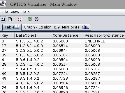
YOUR ANSWER HERE

The Graph tab shows the stem plots of core and reachability distances. We need to increase the Vertical adjustment in the General Settings panel to see the variations more clearly:

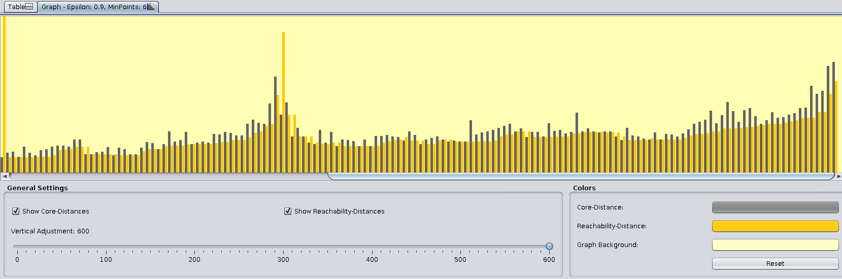
YOUR ANSWER HERE

Change the General Settings to give the reachability plot below:

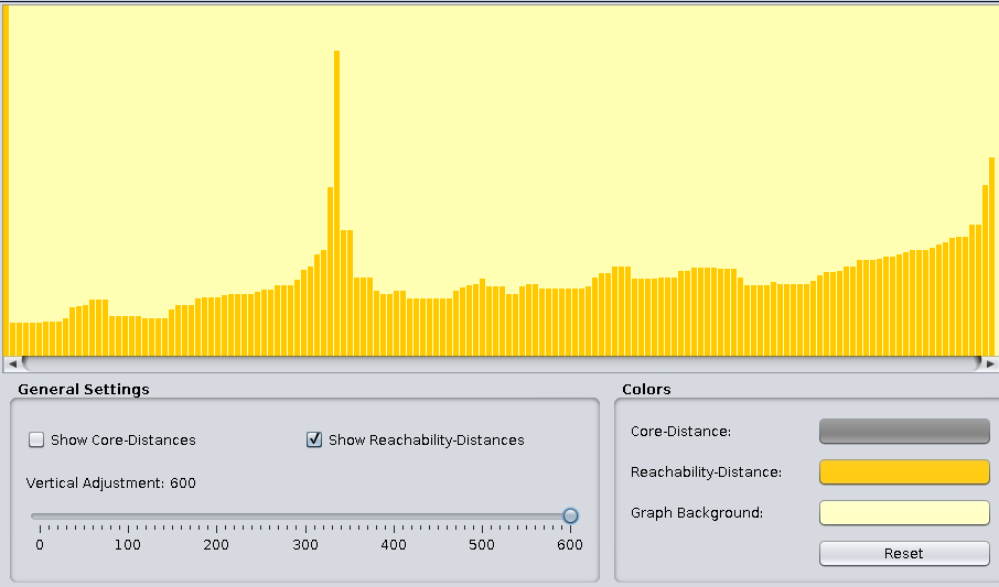
The above stem plot is called the reachability plot.

Note that noise points in DBSCAN may be considered clusters at higher density levels by OPTICS. Since the reachability plot is a 2D representation regardless of the dataset’s dimensions, it allows for easier identification of appropriate thresholds for clusters with varying density levels.

# YOUR CODE HERE
raise NotImplementedError
eps_cl

# hidden tests

# YOUR CODE HERE
raise NotImplementedError
eps_cl

# hidden tests

# YOUR CODE HERE
raise NotImplementedError
error_rate, miss_rate

# hidden tests

%%ai chatgpt -f text
For OPTICS, can we quantify how stable a cluster is, and how likely a point is
a noise point?

%%ai chatgpt -f text
Explain HDBSCAN and compare it with OPTICS. Is HDBSCAN better?